Passenger Fares of the RMS Titanic

Data visualization allows one to easily see patterns and trends that can peak further data investigation and intriguing questions. Follow along as I explore some information regarding passengers of the RMS Titanic through data visualizations in RStudio.

On April 10, 1912, Titanic set sail for the first time with 1,316 passengers onboard. While there has been a lot of discrepancy regarding the number of passengers onboard and the number of passengers that survived, the data I will be using accounts for 887 of the ships passengers.

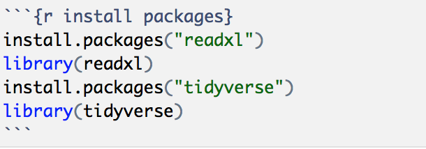
Before we can work with the data, we have to import the dataset into RStudio. Installing R package “readxl” will read data from the Titanic excel file and the “tidyverse”” package will allow me to work with ggplot data visualizations.

Once installed, we will assign the data from the Titanic excel file into the data frame “passengers”.

What’s a data frame you ask? It’s a list of variables with the same number of rows, where each variable is a column of that data frame. In other words, it is used for storing data tables. Let’s now take a look at the names of the variables with colnames() to see what variables we have to work with.

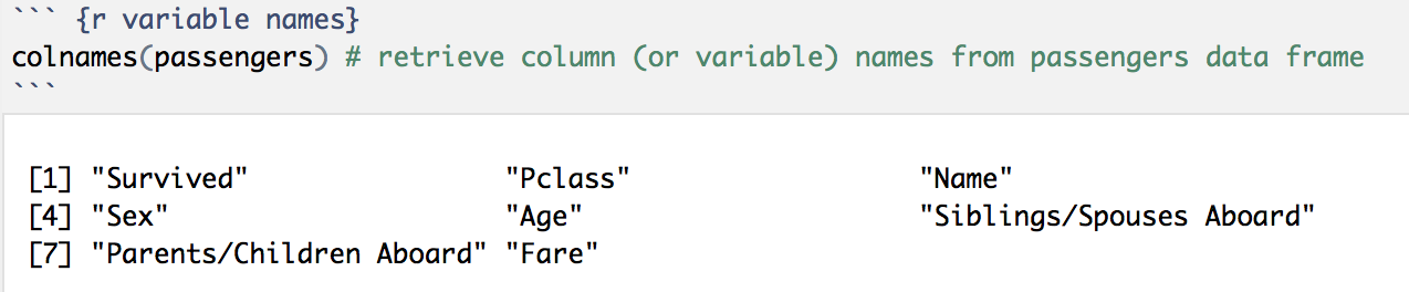
Looking at the variable names in the data set we can see that we have personal passenger information like names, age and gender. We also know whether or not a passenger survived the sinking, what passenger class they were in, what fare they paid and what family members they had onboard. We will focus on age, passenger class and gender to see what, if any, influences they had on the fares that the passengers paid.

Let’s first take a look at a distribution of ages of the passengers on board with a histogram using the hist() function.

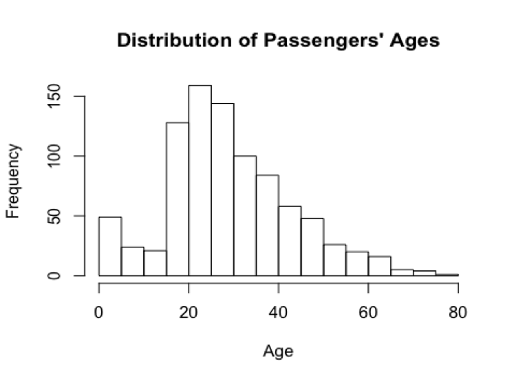
Looking at the distribution of ages, we can see that there were many younger passengers onboard. The average passenger age was 29, while 50 passengers were between the ages of 0 and 5. Only 25% of passengers were over the age of 38, with the oldest person onboard at the age of 80.

These ages are not surprising considering that life expectancy for men in 1912 was 51.5 and 55.9 for women (USA).

How much did it cost to travel? Let’s take a look at the distribution of fares.

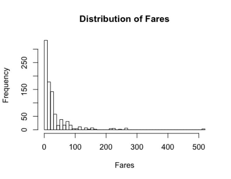
Over 300 passengers paid fares of 10 or less. The average fare was 32.3 and the maximum fare paid was 512.33.

So, did a passenger’s age have any factor on the fare that they paid? Let’s create a scatterplot to see if there was a relationship between passenger age and fares.

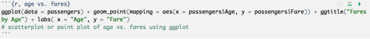
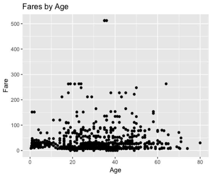
Looking at the scatterplot, we can see that passengers of all ages, paid different fares. The fare a passenger paid was not dependent on age.

It’s more likely that fares depended on passenger class; so let’s examine that.

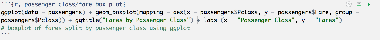
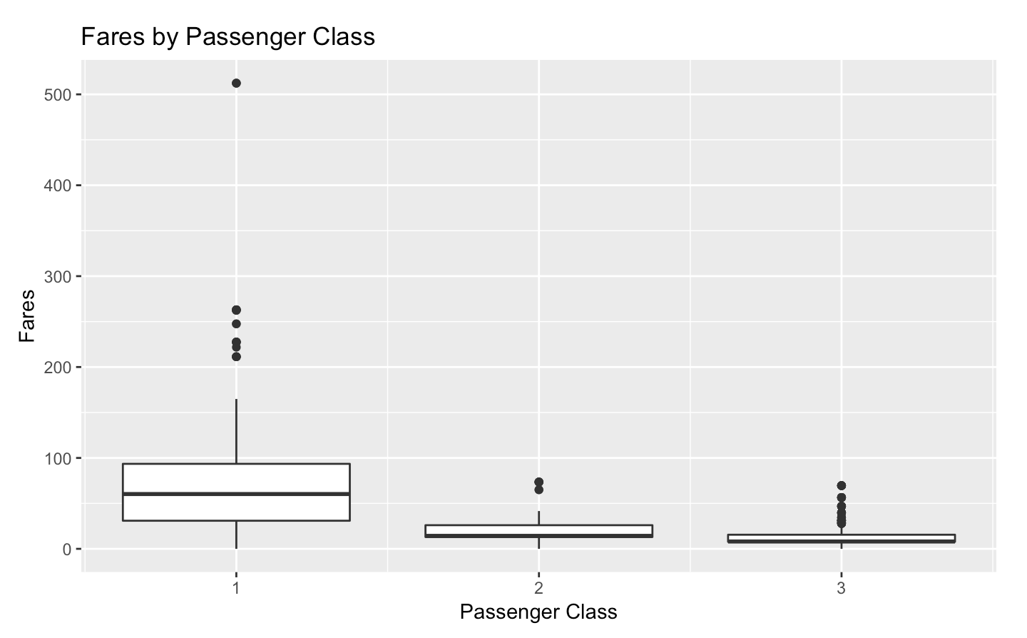
These box plots show that passengers in 1st class had higher fares than passengers in 2nd class and that passengers in 2nd class had higher fares than 3rd class. Comparing the medians and the means of these groups reinforces this. The 1st class mean of 84.15 was higher than both the 2nd class mean of 20.66 and the 3rd class mean of 13.71. Statistical analysis comparing the means among the three groups could confirm this.

Did gender play any role in fares? Let’s first take a look at the split between female and male passengers.

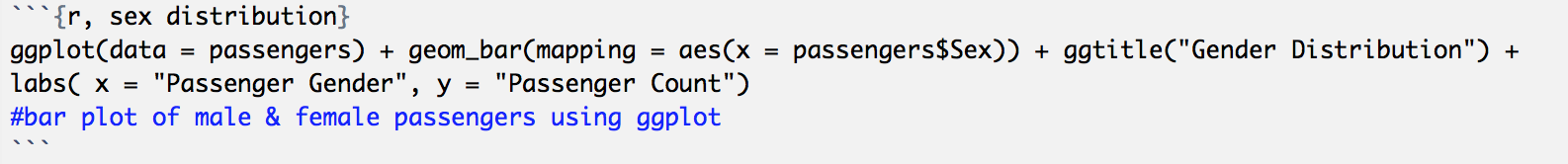
As we can see, more males travelled on Titanic than females. From this selection of data there were 573 males and 314 females.

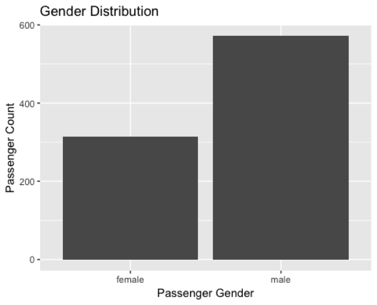
Now, let’s take a look at if gender played a role in fares.

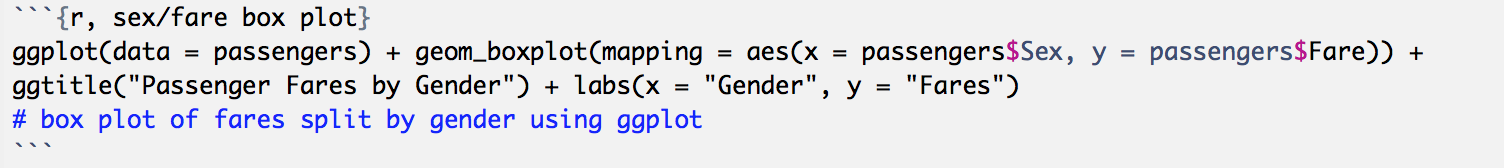
The box plot for female passengers contains a higher median value and a larger 3rd quantile. Both genders had one passenger pay the highest fare, but a large percentage of females paid higher fares in general. To get more concrete evidence of females having higher fares lets reference actual quantiles for these box plots.

Except for the 100th percentile where a female and male passenger paid 512, females were paying more amongst the other quantiles. Females in the 50% quantile paid 23 while males paid 11.13. The average fare was even higher at 44.4 for females and 25.63 for males; another finding that could be confirmed with proper statistical testing.

So far, we have seen that 1st class passengers paid more and that females paid a higher average fare; why was this? Let’s take a look at the break down of females and males between passenger classes.

The bar graph for each passenger class, split by gender, shows that there were more males in all passenger classes. Let’s look at the details.

3rd class had 343 males to 144 females, with 3rd class female passengers paying an average fare of 16.12 while 3rd class male passengers paid an average fare of 12.69.

We can now see clearly why the average fare for female passengers was higher. There were more males paying lower fares, which in turn lowers the mean for that group. 3rd class male passengers also made up 59.8% of all males accounted for in the data set and 38.7% of all passengers accounted for in the data set. Since 59.8% of male passengers were paying lower fares in comparison to the 45.8% of females that paid lower fares, this explains why all females paid an average higher fare.

We see similar trends with 2nd and 1st class passengers.

2nd class had 108 male passengers to 76 female passengers. Females paid an average fare of 21.97, while male passengers paid 13.00.

1st class had 94 females to 122 males, but the average fare that females paid was 106.13 to the 67.23 that males paid. Even the median of 82.66 for females was higher than the median for males at 41.26.

Why was this? The average for females fares across all passenger classes were higher than males’, especially for female passengers in 1st class. Did females in first class have special lodging on board Titanic, or were they charged more simply because they were female? Only further investigation could tell the answer.

I have explored only four of the variables provided in the data set and have already encountered an interesting find and raised several questions, simply through visualizing the data. Where can data visualization take you?

Click below for the full R code.