In today’s world, there is a significant emphasis on applied data science and the utilization of machine learning algorithms to tackle real-life problems. However, amidst this focus, it’s easy to overlook the importance of understanding the underlying principles that drive these algorithms. In reality, grasping the theory and mathematics behind them empowers data scientists to construct even more effective models for practical applications.

That is precisely why I’ve chosen to write this blog post: to dive into the mechanics behind one of the simplest and most foundational machine learning algorithms one encounters – linear regression.

This post will cover:

• A refresher of linear regression
• An overview of linear algebra
• An example in Python showing how to manually solve linear regression

Linear Regression:

Linear Regression is an algorithm used for predicting target values for future or distinct datasets by modeling relationships observed in existing data. It achieves this by fitting a linear equation to the data and minimizing the difference between the predicted values by the model and the actual observed values. The accuracy of the model is determined by the reduction in this difference, known as residual errors. Essentially, the closer the predicted values align with the observed values, the more accurately the model describes the data. Typically, the algorithm iterates through several lines until it identifies the ‘best fit’.

A classic example often used to illustrate the application of linear regression is the Boston Housing dataset. This dataset enables the prediction of the median value of homes in Boston based on various factors such as the average number of rooms, distance to employment centers, pupil-teacher ratio, and more. It is this dataset that I’ll be using as an example and referencing in this post.

Before examining the dataset itself, let’s first examine some foundational theory:

Linear Regression Theory:

Linear regression comes in two forms: simple linear regression, which involves one dependent variable and one independent variable, and multiple linear regression, which incorporates multiple independent variables.

In simple linear regression, the equation takes the form:

y = b_{0 ​}+ b_1​x

Here, y represents the dependent variable we’re trying to predict, x denotes the independent variable, b_0​ signifies the intercept of the equation (the value of y when x=0), and b_1​ represents the slope or coefficient for the independent variable (indicating the average change in y for a one-unit change in x).

This equation extends to multiple linear regression with n number of variables:

y = b₀​ + b₁x₁​ + b_2​x₂​ + … + b_n​x_n​

The objective of linear regression is to determine the optimal values of the intercept and coefficients to minimize the residual errors and generate the ‘best fit’ line.

Here are some assumptions and considerations to keep in mind while working with linear regression:

• The dependent variable must be quantitative. For predicting binary or categorical variables, other methods such as logistic regression or classification models should be used.
• Linearity between the independent and dependent variables is crucial. The linear regression model operates on a system of linear equations, and deviation from linearity can affect model accuracy and lead to biased results.
• Regression analysis relies on normally distributed residuals to accurately estimate standard errors, confidence intervals, and p-values. Thus, residual errors should ideally follow a normal distribution for precise results.
• Multicollinearity arises when independent variables are highly correlated. If two variables contain similar information, it makes it difficult to estimate their individual effects on the target variable. Therefore, it is essential for independent variables to not be correlated or for one of two highly correlated variables to be dropped from the model.
• Autocorrelation occurs when residual errors are correlated with each other, violating the assumption of independent values and leading to inaccurate results. Hence, no autocorrelation is preferred.
• Finally, there’s the assumption that residual errors exhibit homoscedasticity, meaning they have constant variance and don’t vary as the predictor’s value changes. Variance in residual errors could bias test results.

Linear Algebra:

Linear Algebra is the branch of mathematics that deals with linear equations and solving for unknowns within a system of linear equations. Algebraic equations typically involve one or multiple non-numerical or alphabetical variables that require solving.

For example:

3x+3=9
3x=6
x=2

An equation is considered linear if the unknown variable is of the first order; if it involves an exponential variable, it is no longer linear (ie. x²).

Moreover, linear algebra enables us to determine the unknown variables across multiple equations provided that they share identical variables – that they belong to the same system.

Let’s illustrate this concept within the context of the Boston Housing dataset. In linear regression, we aim to model the relationship between independent variables and the dependent variable in the observed dataset to predict new target values when presented with new data. Within this dataset, the dependent variable y, representing the median house value, and several independent variables such as the average number of rooms, allow us to create an equation to solve for y based on the predictor values. With data on multiple houses, we’re dealing with multiple equations. Since these equations model the same house value with identical predictors, they form a system of equations:

These equations should look familiar as they are just the equations for multiple linear regression.

Now remember, our objective with linear regression and this system of equations is to determine the best intercept and coefficients to describe all the data and satisfy all equations within the system of linear equations.

Great, now how do we solve this system of linear equations? Conventional methods such as substitution or elimination are not practical here given that n can be a very large number. Let’s represent the above system of equations in a different format:

Linear regression can be solved by multiplying the independent variables by their unknown coefficients and the equation intercept, which remains consistent across all equations within the system. Utilizing the distributive property of multiplication, we can isolate the unknowns from the independent variables and express the equation as follows:

Hmm… they seem somewhat like vectors and a matrix, don’t they? This implies that we can solve the system of linear equations using matrix inversion! Now, let’s delve into some vector and matrix foundations.

Vectors and Matrices:

Some terminology to get us started:

• A scalar is a value denoted in italics: x
• A vector is an array of numbers denoted with a bold lowercase letter: x (eg. [ x₁ x₂ x₃ ])
• A matrix is a rectangular array of numbers denoted with a bold uppercase letter: X

Common operations that can be done to vectors and matrices include:

• Basic arithmetic: such as element-wise multiplication and addition
• Transposing: converting a vector from row to column or vice versa and flipping a matrix over its main diagonal
• Reduction: this can reduce a vector or matrix down to the sum across all elements
• Dot product: multiplying two vectors based on the corresponding elements and summing the products to produce a scalar value that tells how much the two vectors point in the same direction or how similar they are
• Matrix multiplication: is just a series of dot products to handle multiple arrays

Matrix Multiplication and Matrix Properties:

Matrix multiplication is probably one of the most important concepts in machine learning and therefore it is important to understand matrix multiplication properties.

Matrix-vector multiplication requires that the number of columns in matrix A equals the number of rows in vector x resulting in a product that is a vector with the same number of rows as matrix A. Multiplication just involves taking the dot product of the vector with each row of the matrix:

Matrix-matrix multiplication requires that the number of columns in matrix A equals the number of rows in matrix B producing matrix C with the same number of rows in matrix A and the same number of columns in matrix B. In the example below, A is m x n and B is n x p, so we end up with C which is m x p. Now that we understand matrix-vector multiplication, we can extend this method to matrix-matrix multiplication where we re-write matrix B as a bunch of vectors lined up next to each other.

One other matrix multiplication method I want to cover is multiplying a matrix by its transpose. The transpose of a matrix is simply the matrix flipped over its main diagonal. When we multiply a matrix by its transpose, it produces a matrix with the same number of columns as the original matrix and the same number of rows as the matrix transpose (which should be the same as the number of columns in the original matrix) producing a square matrix:

Above we see A a 3×2 matrix and A^T a 2×3 matrix resulting in a 2×2 matrix.

Now that we have covered the matrix multiplication method, there is one final matrix property you need to understand before we can cover matrix inversion, and how that can help solve a linear system of equations. This property is the Identity Matrix.

The identity matrix is a square matrix (the same number of rows as columns) with only 1s on its diagonal and 0s for every other element, denoted with an italicized I. Note: the identity matrix is a type of special matrix called a diagonal matrix, among other types of special matrices.

Characteristics of the identity matrix are that when a vector is multiplied by an identity matrix the product is just the vector. Similarly, when a matrix is multiplied by the identity matrix, the product is just the matrix.

Matrix Inversion and Solving for Unknowns

This finally brings us to matrix inversion and how we can use it to solve for the unknown intercepts and coefficients in our linear regression model.

An inverse matrix is a matrix such that when multiplied by the original matrix the product of the matrices is equal to the identity matrix. That is, if you multiply matrix A by its inverse matrix A^-1 you have A * A^-1 = I. Let’s look at an example:

Let’s say we have matrices A and A^-1:

Now let’s look at how to multiply these two together to get the identity matrix:

Now, going back to our linear regression equation, we have our median house values, y, our predictors, X, and our unknown intercept and coefficients, let’s call this w: y = Xw.

If we multiply both sides of the equation by X^-1 that gives us: yX^-1 = XX^-1w or just yX^-1 = Iw since a matrix multiplied by its inverse is just the identity matrix. And what happens when we multiply a vector by the identity matrix? We just end up with the vector unchanged. This means that our unknown vector w = yX^-1. We just need to multiply our vector of median house values by the inverse of the predictors’ matrix and we will have the unknowns for the equation that we can use to predict median house value on different data.

Two key limitations of matrix inversion are:

• The columns must not be singular and must be linearly independent. If the lines do not intersect there will be no solution and if the lines completely overlap then there will be infinite solutions.
• The inverse matrix can only be calculated if the number of rows is equal to the number of columns, in other words, it has to be a square matrix. This

That second limitation is a bit of an issue for us because neither our X matrix nor our X^-1 matrix are square, meaning that they are not invertible. Luckily, as we learned earlier in the post, multiplying a matrix by its transpose produces a square matrix. To solve the unknown weights (w = yX^-1) we would need to multiply both X and y by the X transpose for the equation to have the correct dimensions for matrix-vector multiplication. This means our equation looks more like this:

w = yX^T * (X^TX)^-1

This works out because X^T and the inverse of X^T end up canceling each other out which produces another identity matrix, which multiplied by the remainder of the solution, just produces the solution.

Now that we have covered all of the important theories that you need to know… let’s take a look at this in Python!

Matrix Inversion for Linear Regression in Python

As I mentioned at the beginning of the post, we are using the Boston Housing dataset to predict median house values. I will only cover key steps here, so if you would like to see the full code, please view it in my GitHub repository.

The Data:

First, let’s take a look at the data to understand what data we have:

The data variable descriptions are below:

• CRIM: Per capita crime rate by town
• ZN: Proportion of residential land zoned for lots over 25,000 sq. ft
• INDUS: Proportion of non-retail business acres per town
• CHAS: Charles River dummy variable (= 1 if tract bounds river; 0 otherwise)
• NOX: Nitric oxide concentration (parts per 10 million)
• RM: Average number of rooms per dwelling
• AGE: Proportion of owner-occupied units built before 1940
• DIS: Weighted distances to five Boston employment centers
• RAD: Index of accessibility to radial highways
• TAX: Full-value property tax rate per 10,000 USD
• PTRATIO: Pupil-teacher ratio by town
• B: 1000(Bk — 0.63)², where Bk is the proportion of [people of African American descent] by town
• LSTAT: Percentage of lower status of the population
• MEDV: Median value of owner-occupied homes in 1000s USD

Data Exploration:

We first need to explore the data to pick which independent variables we want to use as predictors in our model. For this, let’s take a look at a correlation matrix (using .corr()) of all the variables to see which variables are correlated and which ones are not.

It is useful to examine the data like this because correlation can help us pick variables that are in linearity with the dependent variable MEDV, but that are also not highly correlated with each other. This helps satisfy two assumptions of linear regression: linearity and no multicollinearity.

Based on the above correlation matrix, variables such as RAD and TAX are highly correlated with each other, as well as, DIS which is highly correlated with several variables, so let’s not use either of those.

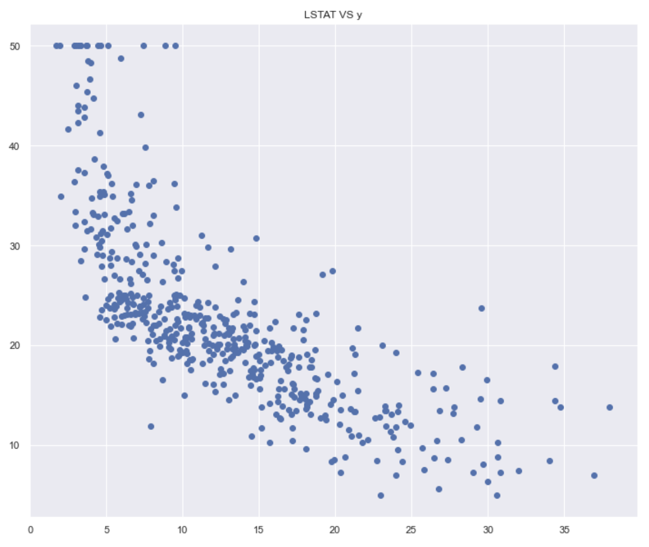
RM and LSTAT have the highest correlations with MEDV and are not too correlated with each other, so let’s use these for now. We can also analyze linearity by plotting each predictor by y and visually seeing how linear the data is:

Data Preparation:

Before modeling, we need to prep the data. First, we need to convert our X table and y column to arrays which can be achieved by using the numpy library (np). Numpy also allows us to do a lot of key operations when it comes to handling matrices and vectors which you will see below.

Second, while we have our y vector, X matrix, and w vector since one of the weights in our w vector is the equation intercept and there is no variable corresponding to the intercept in our X matrix, we need to add a column of 1s to our X matrix so that once multiplied, those values are accounted for:

#adding ones to X and converting X to array (our matrix)
one = np.ones((len(X),1))
X = np.append(one, X, axis=1)
X

This code turns the X table into an X matrix:

output:
array([[1.   , 4.98 , 6.575],
       [1.   , 9.14 , 6.421],
       [1.   , 4.03 , 7.185],
       ...,
       [1.   , 5.64 , 6.976],
       [1.   , 6.48 , 6.794],
       [1.   , 7.88 , 6.03 ]])

And let’s also convert the y column into a column vector array:

#reshape Y to a column vector
y = np.array(y).reshape((len(y),1))
#preview of the top 10 values
y[:10]

Output:
array([[24. ],
       [21.6],
       [34.7],
       [33.4],
       [36.2],
       [28.7],
       [22.9],
       [27.1],
       [16.5],
       [18.9]])

Finally, let’s confirm the X has 3 columns, y has one column and both have the same number of rows:

print(X.shape)
print(y.shape)

Output:
(506, 3)
(506, 1)

Modeling:

First, we need to split our data into our training data and test data. The training data is the data we will use to find the unknown weights, and we will use the weights to build a model to predict median house values for test data.

We typically need more data for training, so here is a 70-30 split of the data:

from sklearn.model_selection import train_test_split

X_train, X_test, y_train, y_test = train_test_split(X, y, test_size = 0.3, random_state = 111)
print(X_train.shape)
print(X_test.shape)
print(y_train.shape)
print(y_test.shape)

Output:
(354, 3)
(152, 3)
(354, 1)
(152, 1)

Now we can make our model in Python. Remember the equation that we have to solve is:

w = yX^T * (X^TX)^-1

This is really easy to do with numpy. We can use np.dot() to multiply, .T for the matrix transpose, and np.linalg.inv() to calculate the matrix inverse. Putting this all together:

w = np.dot((np.linalg.inv(np.dot(X_train.T,X_train))), np.dot(X_train.T,y_train))

And this one line of Python code gives us our unknown weights:

w

Output:
array([[ 2.43370426],
       [-0.70314558],
       [ 4.57890942]])

The first value here is the coefficient of the intercept which is 2.43370426. This value gives us the average median house value where both ‘RM’ and ‘LSTAT’ are zero. Since the median house value is in the 1000s, this means the average median house value is $2,433.70.

The second value, -0.70314558, is the coefficient for ‘LSTAT’, meaning that for a 1 unit change in the percentage of lower status among the population, there is an average decrease in median house value by $7,032. This makes sense that houses will have lower value if more people of a lower financial status live in the area and this is aligned with both variables’ negative correlation with each other from our data exploration.

The third value, 4.57890942, is the coefficient for ‘RN’, meaning that for a 1 unit change in the average number of rooms, there is a $4,832 average increase in median house value. This makes sense since more rooms mean a more expensive house and is aligned with the variables’ positive correlation with each other from our data exploration.

Predict and Analyze:

Now we can predict MEDV on the test data with the new weights to evaluate the model:

y_preds = np.dot(X_test, w)

Finally, let’s calculate some evaluation metrics to analyze the model results:

#calculating mean absolute error
MAE = np.mean(np.abs(y_preds-y_test))

#calculating root mean square error
MSE = np.square(np.subtract(y_test,y_preds)).mean() 
RMSE = math.sqrt(MSE)

#calculating r_square
rss = np.sum(np.square((y_test- y_preds)))
mean = np.mean(y_test)
sst = np.sum(np.square(y_test-mean))
r_square = 1 - (rss/sst)

print(MAE)
print(MSE)
print(RMSE)
print(r_square)

Output:
4.440107104057758
39.21051019278403
6.26182962022954
0.6046389447452969

A low MAE and RMSE, and a high MSE are good indicators of accurate predictions.
The R square value of 60% indicates that 60% of the variance in y is explained by the model, which is a pretty good outcome. There is definitely room for improvement, but that is beyond the scope of the post.

Summary

Thank you so much for following along on this really long post. In this post, we covered the foundations of both linear regression and linear algebra with a focus on linear systems of equations and matrix and vector properties to manually solve for the unknown weights in linear regression and predict new Boston Housing house values.

I hope you now understand just how linear regression, linear algebra and matrices are all related.