I recently completed an online course on A/B Testing and as someone who works with websites, this was something I wanted to try out for myself. In this post, I practiced doing an A/B test in R while thinking through the important considerations that need to be made in order to have a successful test. Note: I have not gone into any detailed statistics here.

If you want to follow along, click here for my source code and access to my GitHub repo with the datasets used.

*Full disclosure, I was not able to find a data set to use, so I created a data set for this A/B test, as it is solely being used for the purpose of practicing.

What is an A/B Test?

An A/B test compares the performance of varying webpage designs. Webpage variations can be anything from changing an image, to the Call-To-Action button or the text on the page.

When it comes to the performance that you’re measuring, an A/B test can be used to compare metrics like conversion rates, engagements, drop-off rate, time spent on website and more. For this post, I created a fictional scenario in which I paid attention to the number of conversions between two versions of a webpage.

Meet KeepKool

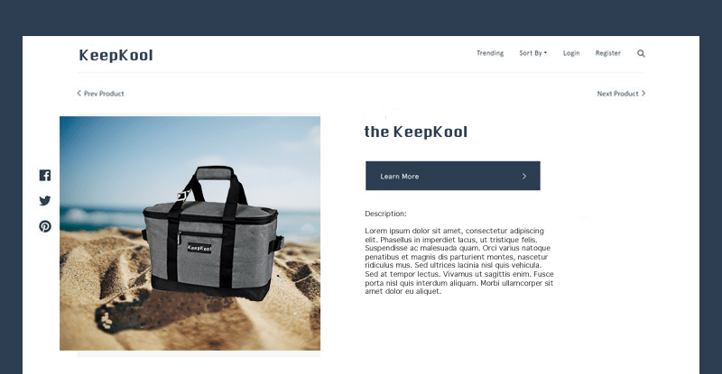
Imaginary company “KeepKool” sells beach cooler bags and is deciding whether or not to update the image used on their product page for their classic product “the KeepKool”. The hope is that using a more engaging photo will get visitors to convert more (click “Learn More”) on the product page. The current product page has a staged photo of the cooler bag with a gray background and they want to update the image to show the cooler actually at the beach.

Original Webpage:

Variant Webpage:

KeepKool already made the variant of the webpage live for the month of May 2019 to see if there was a difference between the number of conversions on the original webpage versus the variant webpage with 50% of visitors seeing the original and 50% of visitors seeing the variant. The reason they chose to do this in May is because this is the start of the summer when people tend to engage more on the site. We can see this from the average number of conversions by week for “the KeepKool” product page depicted below:

KeepKool found that the average number of conversions for the variant was higher than that of the original; 8.69 for the variant and 4.76 for the original. However, since they did not methodologically plan out how long to keep the page live for or how much data to collect, it did not make sense to run a significance test on the data collected to see if this increase was statistically significant. KeepKool doesn’t want to permanently change the image until they know that the difference is statistically significant. Therefore, KeepKool decided to run a proper A/B test.

Things to Consider Before Running an A/B Test

Before running an A/B test, there are several things to consider. I have these considerations listed below along with what I will be doing for each one in this experiment.

• Choose one variable to change (image)
• Think about potential confounding factors (visitors accidentally seeing both versions of the webpage, increase in demand for the product)
• Create a “control” and an “experiment” (the “original” and the “variant” webpages)
• Determine the goal (to see if the difference between the mean conversions of both variations is statistically significant)
• Determine Hypotheses:
  • Null Hypothesis: There is no statistical significant difference between the mean conversions of the Control and Experiment webpages.
  • Alternative Hypothesis: There is a statistical significant difference between the mean conversions of the Control and Experiment webpages.
• Decide your significance level (default p-value is below alpha (0.05))
• Determine what statistical test/distribution you need (to be determined below)
• Determine your sample size (to be determined below)

What Statistical Test/Distribution do I Need?

One of the first steps before doing an A/B test is to what know test you are going to use for your analysis. I plan to run a Generalized Linear Model (glm) regression. A regression can tell you what effect and if the effect on a dependent variable by an independent variable is statistically significant. Glm is a flexible version of the ordinary linear regression and allows you to adapt your regression for different statistical distributions.

This is important because the data being collected in this case is the number of conversions. Since a conversion, like a visit or a click, is considered count data, we are limited to distributions that can account for discrete data. A regular linear regression is limited to data with a normal distribution, but glm will allow me to use a Poisson distribution which accounts for discrete data. So, I plan to use a Poisson regression.

Now that I know what kind of distribution I need to consider when doing my statistical significance test, I can now determine how much data I need to collect as part of the experiment. Let’s learn about power analysis.

Power Analysis

Power analysis is normally conducted before data collection to determine the smallest sample size that is suitable to detect the effect of a given test at the pre-decided level of significance. This can be helpful for marketers who don’t have a lot of time or money to run a long experiment.

The kind of power analysis test that is used is dependent on the distribution of the data. I already determined that the data collected will best be accounted for by a Poisson distribution, therefore, I will use the wp.poisson function in the WebPower package for my power analysis:

wp.poisson(n = NULL, 
           exp0 = 4.758621, 
           exp1 = 0.8260868, 
           alpha = 0.05,
           power = 0.8, 
           alternative = "two.sided",
           family = "Poisson", 
           parameter = 1)

In the wp.poisson function, the arguments are:

• n – sample size
• exp0 – the base rate under the null hypothesis
• exp1 – the relative increase of the event rate
• alpha – the significance level for test; typically set to 0.05
• power – statistical power; typically set to 0.8
• alternative – direction of the alternative hypothesis
• family – distribution of the predictor or independent variable
• parameter – corresponding parameter for the predictor’s distribution

Since I am trying to find the sample size, I leave the “n” argument as “NULL” so that the function will let me know what this value should be. I set exp0 as the average number of conversions for the original webpage from the baseline data and the exp1 as the relative increase between the average numbers of conversions between the original and variant webpage baseline data.

As a result, wp.poisson told me that I need a sample size of 65 data points; that’s 65 data points for both conditions; the Control (original) page and the Experiment (variant) page.

Now, KeepKool can run a proper A/B test. Because their baseline data was from May 2019, in order to account for the same demand and seasonality and reduce confounding effects, they had to wait until May 2020 to run the experiment and collect data. Additionally, similar to their baseline test, 50% of visitors saw the Control webpage and 50% saw the Experiment webpage at random. Let’s examine the data below.

Analyzing Experiment Data

First, let’s look at a plot of number of conversions between the Control and the Experiment:

Similar to the baseline data, it seems that Experiment page had more conversions throughout the month. Comparing the means, 12.58 for the Control and 16.00 for the Experiment, confirms this.

Before running the Poisson regression, I decide to look at the variances for both the Control and Experiment variables, since one of the requirements for the Poisson regression is that the variance be equal or similar to the mean. The variances for the Control and Experiment variables are 76.78 and 68.47, respectively. Clearly not close to their means. Therefore, I will use the Quasi-Poisson regression instead, because it is the generalized version of the Poisson regression which can be used when the variance is greater than the mean.

Now, let’s look at glm regression for the Quasi-Poisson distribution to test the significance of the Experiment variable’s effect on conversions, where tidy() is a function that cleans up the output:

glm(Conversions ~ Condition, family = "quasipoisson", data = experimentData) %>%
  tidy()

From the regression output, the estimate for the Experiment Condition is positive meaning that the Experiment webpage increases conversions; this confirms what was observed in the baseline data. The p-value for the Experiment Condition is less than 0.05. This means that there is a statistical significant difference between the mean conversions of the Control and Experiment webpages. Therefore, we can reject the Null Hypothesis, and KeepKool can permanently change the image on their webpage in order to get more conversions.